4. Orthogonality
4.1. Orthogonality of the Four Subspaces
여기 링크에 Linear Algebra의 다른 fundamental theorem도 함께 있으니 한번 봐보자.
Those four fundamental subspaces reveal what a matrix really does.
Def.
Orthogonal subspaces
Two subspaces V and W of a vector space are orthogonal if every vector v in V is perpendicular to every vector w in W.
vt w=0 for all v in V and all w in W.
Observations.
Orthogonality is impossible when dim V + dim W > dim whole space.
Zero vector is the only vector where null space meets row space, also 90 degree. And so do left null space and column space.
Proposition.
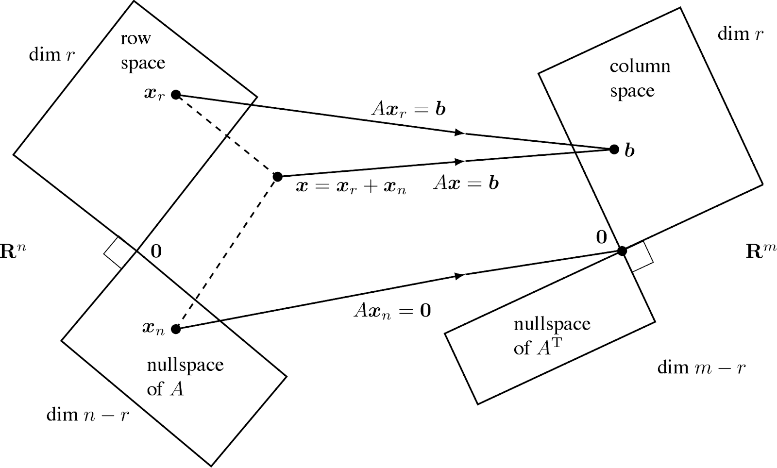
The nullspace N(A) and the row space C(At) are orthogonal subspaces of Rn.
The left nullspace N(At) and the column space C(A) are orthogonal in Rm.
Proof.
Practical
Mathematical
Orthogonal Complements.
Those fundamental subspaces are not only orthogonal, they are orthogonal complements.
Def.
The orthogonal complement of a subspace V contains every vector that is perpendicular to V. This orthogonal subspace is denoted by V perp.
있는데, orthogonal complement에서는 complement가 가지는 의미가 매우 중요하다.
Fundamental Theorem of Linear Algebra, Part 2.
N(A) is the orthogonal complement of the row space C(At) in Rn.
N(At) is the orthogonal complement of the column space C(A) in Rm.
Part 1 gave the dimension of the subspaces. Part 2 gives the 90 angles between them.
The point of “complements” is that every x can be split into a row space component xr and a nullspace component xn. When A multiplies x=xr+xn, above fig shows what happens:
The nullspace component goes to zero: Axn=0
The row space component goes to the column space: Axr=Ax.
Combining Bases from Subspaces
Some valuable facts about bases.
Any n independent vectors in Rn must span Rn. So they are a basis.
Any n vectors that span Rn must be independent. So they are a basis.
When the vectors go into the columns of an n by n square matrix, here are the same two facts.
If the n columns of A are independent, they span Rn. So Ax = b is solvable.
If the n columns span Rn, they are independent. So Ax = b has only one solution.
Proof.
Uniqueness implies existence and existence implies uniqueness.
Proposition.
Given a matrix with bases for the fundamental subspaces,
r, n-r vectors of the row space and the nullspace are independent.
r, m-r vectors of the column space and the left nullspace are independent.
Proof.
If a combination of all n vectors gives xr+xn=0, then xr=-xn is in both subspaces. So xr=xn=0, which proves independence of the n vectors together.
4.2. Projections
Two questions.
Show that projections are easy to visualize.
Projection matrices - symmetric matrices with P^2=P. The project of b is Pb.
Find the combination p = x^hat dot a = x^hat1 a1 + … x^hat n an closest to a given vector b. ⇔ We are projecting each b in R^m onto the subspace spanned by the a’s, to get p.
어떤 subspace 내에 있는 vector를 projection 하는 문제는 위 고민으로부터 왔다. 이 문제를 풀기 위한 핵심적인 아이디어는 geometry로부터 온다. 주어진 subspace와 error vector가 orthogonal 한 성질을 이용한다.
Projection Onto a Line
Projection Onto a Subspace
A^t A x^hat = A^t b
p = A x^hat = A(A^tA)^-1 A^t b = Pb
At (b-Ax^hat)=0 이므로 error vector e는 left null space (N(At))이다.
정리.
AtA is invertible if and only if A has linearly independent columns.
Proof.
We will show that AtA has the same null space as A.
The columns of A are independent -> AtA invertible
Ax=0.
A has linearly independent columns, so null space is zero vector. So does AtAx=0.
AtA invertible(has independent columns) -> The columns of A are independent.
AtAx=0.
xtAtAx=(Ax)t(Ax)=(Ax)^2=0
So N(AtA)=N(A), And if N(AtA) has independent columns, so does A.
4.3. Least Square Approximations
https://en.wikipedia.org/wiki/Least_squares
The method of least squares is a standard approach in regression analysis to approximate the solution of overdetermined systems (sets of equations in which there are more equations than unknowns) by minimizing the sum of the squares of the residuals made in the results of every single equation.
https://en.wikipedia.org/wiki/Regression_analysis
In statistical modeling, regression analysis is a set of statistical processes for estimating the relationships between a dependent variable (often called the 'outcome variable') and one or more independent variables (often called 'predictors', 'covariates', or 'features'). The most common form of regression analysis is linear regression, in which a researcher finds the line (or a more complex linear combination) that most closely fits the data according to a specific mathematical criterion.
Ax=b의 해가 없는 경우가 있다. ⇔ too many equations ⇔ overdetermined systems ⇔ e=b-Ax를 항상 0일 수는 없다.
가장 작은 e를 얻었을 때, x hat은 least square solution이다.
Here is a short unofficial way.
when Ax = b has no solution, multiply by At and solve AtAx^hat = Atb. we must connect projections to least squares.
Minimizing the Error
By geometry
https://ccrma.stanford.edu/~jos/sasp/Geometric_Interpretation_Least_Squares.html
https://www.youtube.com/watch?v=oWuhZuLOEFY
The nearest point is the projection p.
By algebra
Every vector b=p(in a column space)+e(in a nullspace of At).
Ax=b=p+e i impossible, Ax hat is solvable.
E = norm(Ax-b)^2=norm(Ax-p)^2+norm(e)^2.
By calculus
Most functions are minimized by calculus. The graph bottoms out and the derivative in every direction is zero. ⇔ continuous, multivariate function 내에서 convex 한 (or locally optima) point가 존재한다.
In least square approximation, a function is given f(x1, x2), so we can solve by calculating partial derivatives of x1, x2 is 0. ⇔ AtAx^hat = Atb.
Partial derivatives ⇔ AtAx^hat = Atb? (not proven in the book)
The Big Picture

In the figure 4.3, x was split into xr+xn. There were many solutions to Ax=b. In this section, the situation is just the opposite.There are no solutions to Ax=b.
Instead of Ax=b, we solve Ax hat =p
N(A) is a zero vector - with independent columns. AtA is invertible. The equation AtAx hat=Atb fully determines the best vector x hat.
Chapter 7 will have the complete picture - all four subspaces included. x = xr + xn, b = p + e.
Fitting a Straight Line
Fitting a line is the clearest application of least squares.
Fitting a Parabola
A system is non-linear, but we can solve an optimized least square approximation for three variables.
4.4. Orthogonal Bases and Gram-Schmidt
https://en.wikipedia.org/wiki/QR_decomposition
http://www.seas.ucla.edu/~vandenbe/133A/lectures/qr.pdf
https://m.blog.naver.com/PostList.nhn?blogId=ldj1725&categoryNo=6&logCode=0
https://web.calpoly.edu/~brichert/teaching/oldclass/f2002217/solutions/solutions11.pdf
This section has two goals.
See how orthogonality makes it easy to find x hat and p and P.
Construct orthogonal vectors.
Def.
The vectors q1, …, qn are orthonormal if
qit qj = 0 when i/=j and 1 when i=j.
A matrix with orthonormal columns is assigned to the special letter Q.
The matrix Q is easy to work with because QtQ=I.
Q is a rectangular, Qt is only an inverse from left.
Q is square, QtQ=I means that Qt=Q^-1: transpose=inverse.
Examples of orthogonal bases.
Matrices for rotation, permutation, reflection.
정리.
If Q has orthonormal columns QtQ=I, it leaves lengths unchanged:
Same length: norm(Qx)=norm(x) for every vector x.
Q also preserves dot products (Qx)t(Qy)=xtQtQy=xty.
Projections Using Orthogonal Bases: Q Replaces A.
Projection을 구하기 위한 수식에서 A가 orthonormal 하다면 AtA=QtQ=I이므로 수식은 간단해진다.
Important case: When Q is square and m=n, the subspace is the whole space. Then Qt=Q^-1 and x hat = Qtb.
The Gram-Schmidt Process
앞서 살펴본 projection, least square approximation에 AtA 연산이 들어가므로 A가 orthonormal bases matrix인 Q가 된다면 계산 상의 이점이 있다.
For this to be true, we had to say “If the vectors are orthonormal”. Now we find a way to create orthonormal vectors.
(Gram-Schmidt 수식)
Subtract from every new vector its productions in the directions already set.
The Factorization A=QR
Since the vectors a, b, c are combinations of the q’s (and vice versa), there must be a third matrix connecting A to Q. This third matrix is the triangular R in A=QR.
(R matrix 수식)
Also R=QtA.
This non-involvement of later vectors is the key point of Gram-Schmidt:
The vectors and A and q1 are all along a single line.
The vectors a, b and A, B and q1, q2 are all in the same plane.
The vectors a, b, c and A, B, C and q1, q2, q3 are in one subspace (dimension 3).
정리.
R is invertible, since diag(R)/=0.
최종적으로 A = QR 식을 통해서 least square approximation을 간단하게 구할 수 있다. 또한 책에서 소개한 modified Gram-Schmidt 는 mn^2 time에 Q, R을 구할 수 있다.
No comments:
Post a Comment